November 2011 – How to remember math without really trying

How to remember what Gauge Theory’s about without really trying

November 12, 2011July 30, 2013Leave a comment

In physics, gauge theories are theories of fields. The fields can’t be seen, but they give rise to observables. It’s the observables we measure directly. The fields can be configured in different ways and all these different ways are connected by symmetries. These different configurations give the same observables.

The fact that the observables don’t change is called gauge invariance.

Imagine Mario on a planet. The planet has round stones on the surface and each stone has a pink line pointing in a certain direction. The pink line is a measurement of some potential.

Luigi is on a similar planet, same size, same stones, same everything. Mario wants to tell Luigi what direction the pink lines are pointing on his planet.

So he fixes a flag on the ground. (He’s agreed with Luigi where the flag should be located).

Then Mario draws yellow lines from the centre of the stones in direction of the flag.

What he has done by planting the flag in the ground is fix a gauge.

Now Mario can read off the angle between the yellow and the pink lines and send the information to Luigi. (They will also need to agree which way round they are measuring things – clockwise or anticlockwise).

Now what if Mario moves the flag?

The pink lines are still in exactly the same position. They haven’t changed and the wind hasn’t changed.

But the flag is in a different position. The gauge has been changed. So Mario has to draw new yellow lines. Then he measures new angles.

The wind is an observable. The flag fixes the gauge. The observables are invariant under the gauge transformation. This invariance under the transformation is called a symmetry. The gauge transformation in this case is not global – Mario can’t simply add the same amount to each angle when he moves the flag to get the new co-ordinate reading. The transformation is local – it varies place to place, but that doesn’t mean it’s arbitrary.

We can add a few more terrifying terms from physics – the planet is the base space. The stones are a circle bundle. The fibre of the circle bundle are all the possible directions the yellow lines could point in. The yellow lines they actually point in are a section of the circle bundle.

The base space doesn’t have to be a planet. It could be anything. It could be a line. And instead of circular stones on the surface of the planet, we could have lines rising upwards. Then we would have a comb.

Or something like it.

A section of the comb might look like this.

Which should remind you of a graph of a function because that what it is.

So a gauge theory is a field theory and theory will involve group actions on fibre bundles.

The simplest example of a gauge theory in physics is electromagnetism.

The electromagnetic field is the field for the electron. We can’t measure the electromagnetic field directly.

If we split the field into its electric and magnetic parts, the electromagnetic potentials V and A are not observable.

The electric field, E, and magnetic field ,B, are observable. We can measure the electric field by setting up a charged ball and an oppositely charged plate and measuring how fast the ball accelerate towards the plate. We can see the magnetic field when we drop iron filings near a magnet and they form themselves into patterns. Electric fields move charges. magnetic fields deflect moving charges. Place a magnet next to a cathode ray TV screen to see this. It’s natural to think of these fields as vector fields.

And then it is equally natural to think these direction and length of all these vectors are the acceleration at which a small mass would fall down a well. The wells are the potentials.

Only the difference in potential is physically measurable.

To model electromagnetism, we set up a complex line bundle on spacetime. Every point in spacetime has a line of complex numbers growing out of it. They are different lengths, like our damaged our comb. We set a gauge and use this gauge to measure off the potential V.

How to remember the Lorentz Transformations without really trying

November 9, 2011February 4, 2012Leave a comment

There are 2 main formulations of Special Relativity.

In Einstein’s original formulation, he postulated that the speed of light (c) remains the same in all inertial frames (and that the laws of physics remain the same in each inertial frame.)

He derived the Lorentz Transformations using what, to me, are rather tortuous arguments involving clocks, moving trains, bombs and so on. It’s also the way Feynman does it in “Six Not-So-Easy Pieces.”

You can see it done here and here if you like that kind of thing.

The Transformations, when they are finally produced, are usually written in the form :

$x' = \dfrac {x-ut}{\sqrt{1-u^2}}$

$t' = \dfrac {t-ux}{\sqrt{1-u^2}}$

$y' = y$

$z' = z$

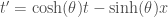
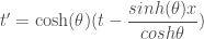
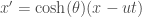
Where $u^2$ is $\dfrac {v^2}{c^2}$ (c being the speed of light, v the relative velocity of 2 observers).

After they’ve been derived in this way it really is necessary to learn them, because you sure as hell aren’t going to have time to derive them like this from first principles to order.

Fortunately, however, Minkowski came along after Einstein and made everything much clearer. He gave an alternative derivation of Special Relativity, which gives us a much more intuitive way to derive the equations from first principles.

Minkowski postulated that spacetime is a 4-dimensional manifold with Minkowski inner product, signature (−,+,+,+).

This was his sole postulate.

The fact that c is constant in all inertial frames drops out as a direct consequence of the way the Minkowski inner product is defined. When a object travels at the speed of light in any reference frame, its interval is 0. The interval, you will recall, is a kind of “distance” on our manifold. The sign of the interval squared indicates whether 2 events can be casually related or not. Our object travelling at light speed is on the edge of the light cone illustrated below. If its interval is 0 in one frame, it’s 0 in all. Hence all observers have the same value for c. (So I suppose you could put it backwards and say that the Minkowski inner product takes the form it does so that c can remain constant in all reference frame.)

1. Recall the basic trig identity, ${\cos \theta }^2 + {\sin \theta}^2 =1$ .

2. Recall there is a hyperbolic equivalent. The only difference between the usual identity and the hyperbolic equivalent is a change of sign. ${\cosh \theta }^2 - {\sinh \theta}^2 =1$ .

3. As a consequence, in a desperate effort to find a transformation that might preserve the interval, write down a pleasing looking matrix.

$\displaystyle \begin{pmatrix} \cosh \theta & - \sinh \theta &0&0\\ - \sinh \theta & \cosh \theta &0&0 \\ 0&0&1&0\\ 0&0&0&1\end{pmatrix}$

This is the inverse of a Lorentz boost. It is simple to remember, much simpler than all the stuff with travelling clocks and bombs on trains. (It’s an inverse so we can write v instead of -v in our Transformations.) Lorentz boosts (and their inverses) preserve the spacetime interval.

4.. Now use this matrix to transform our original co-ordinates.

$\displaystyle \begin{pmatrix} t', & x', &y',&z'\end{pmatrix} = \begin{pmatrix} \cosh \theta & - \sinh \theta &0&0\\ - \sinh \theta & \cosh \theta &0&0 \\ 0&0&1&0\\ 0&0&0&1\end{pmatrix} \begin{pmatrix} t \\ x \\ y \\ z\end{pmatrix}$

5. Multiply through. We get

$t' = \cosh (\theta)t - \sinh (\theta)x$

$x' = -\sinh (\theta)t + \cosh (\theta)x$

6. Rewrite both equations as

$t' = \cosh (\theta)(t - \dfrac{sinh (\theta)x}{cosh \theta})$

and

$x' = \cosh (\theta)(x - \dfrac{sinh (\theta)t}{cosh \theta})$

7. Define $u =tanh \theta = \dfrac {sinh \theta}{cosh \theta}$ .

This is the rapidity.

The equations in 6 above now read:

$t' = \cosh (\theta)(t - ux)$

and

$x' = \cosh (\theta)(x - ut)$

8. A little jiggling about gives $\cosh(\theta)= \dfrac{1}{\sqrt{1-u^2}}$

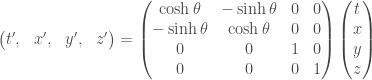
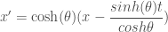
9. So substituting for $\cosh \theta$ in our 2 equations we have

$t' = \dfrac {t-ux}{\sqrt{1-u^2}}$

$x' = \dfrac {x-ut}{\sqrt{1-u^2}}$

as required.

So what we have really done is view the Lorentz transformation as a hyperbolic rotation of coordinates in Minkowski space, (space-time) where the parameter $\theta$ represents the hyperbolic angle of rotation, often referred to as rapidity. (That bits from Wikipedia, as is the picture below of a hyperbolic rotation)

This hyperbolic rotation is what happens in space-time (or Minkowski) diagrams when the axes are squished together to introduce a new frame of reference.

The rotation is hyperbolic because of the minus sign in our Minkowski inner product, which leads us to the hyperbolic trig identity, which leads us to the matrix, which leads us to the Transformations.

How to remember Fourier Series without really trying

November 6, 2011November 10, 20111 Comment

Imagine you are in a room alone. You have a piece of paper in front of you with a cross marked on it. Beside you is a phone. You pick up the phone and, strangely, it’s your friend Stan on the line.

“Hi Stan,” you say.

“Hi,” says Stan. “How are you doing?”

“Not so good,” you say. “I’m in a room on my own with a piece of paper in front of me. There’s a small cross marked on it.”

“Where?” says Stan.

“Where’s the room? I have no idea.”

“No. Where’s the cross? Because I’m in a room on my own too and there’s a blank piece of paper in front of me. I thought it would be nice if I could put a cross on it in the same place as yours.”

You feel sorry for Stan. You want him to put a cross on his paper too. And because yours looks so good, positioned where it is, you want his cross to be in exactly the same place on his paper as the cross is on yours.

How do you do it?

Well, you might tell him to orient the paper so that longest side is closest to him. And then you might tell him to move his finger, along the bottom side of the paper and to stop halfway along, say, if your cross is halfway along. Then you would tell him to move his finger up, say a quarter of the length of the vertical side of the paper, if that’s where you cross was positioned. Then he would mark the cross and when the door between your two rooms was opened and you were able to compare pieces of paper they would look pretty similar.

So what is it you actually did?

You had a 2-dimensional space (the sheet of paper). This is a part of the Euclidean Plane ${\Bbb R}^2$ . You created the bases of a co-ordinate system (you turned the paper length-wise towards you and told Stan up is away from you and across is to the right. The 2 basis axes were orthogonal (fancy way of saying perpendicular to each other). Where the 2 axes met (the bottom left hand corner of the paper) was fixed as the origin of the co-ordinate system. Then you gave him the co-ordinates of the cross in the basis you had chosen. You could have chosen a different basis but this one was fine. The cross could have been on any part on the paper and you could have told Stan where it was unambiguously.

We define a vector, $v$ as an arrow from the origin of our space to the point we are interested in. Then we can call the vector from the origin (the bottom, left corner of the paper) to the bottom right corner of the paper $e_1$ . We define the vector from the origin to the top left corner as $e_1$ . Then the bases vectors for our piece of paper are $e_1, e_2$ . We told Stan the position of the cross by giving him $v$ , expressed as the proportional sum of the basis vectors (in this case $\dfrac{1}{2} e_1 + \dfrac {1}{4} e_2$ ).

Now, Stan is back in his room and you are back in yours. There is a fly hovering above your head. It is bizarre. It’s staying still, hovering, but in one spot. You pick up the phone to Stan. He has to be told.

“So where exactly is this fly?” Stan says.

Well, this is going to be a bit more of a challenge. Fortunately you have a tape measure on you so you are able to tell Stan the fly is positioned exactly 7 meters along from the corner of the room where the phone’s plugged in (which you have defined as your origin), straight up 3 meters and straight across 2. Stan puts the phone down a happy man. He has the exact picture of where the fly is.

So, again, what did you do?

The room is 3-dimensional i.e. you are in ${\Bbb R}^3$ . You picked on origin and a co-ordinate system as before. You fixed it so the axes (the edges of the room) were orthogonal to each other. This the most logical thing to do if you want your bases vectors to sweep out the entire space. You told Stan the position of the fly in terms of the bases you had chosen. The fly could have been anywhere and you would have unambiguously told Stan where it was.

Now here’s where Stan gets very confused. Because we’re mathematicians, there’s nothing to stop us doing the same thing in 4-dimensions. Or 5-dimensions. Or 567889 dimensions. Or an infinite number of dimensions.

The more dimensions we go up, the more information we have to convey to fix a position. By the time we’re at 567889, that’s 567889 co-ordinates we have to specify to fix one position. Or alternatively, just knowing where exactly one fly is in 567889-dimensional space gives us an enormous amount of information.

When we are in 2 or 3 dimensions we have an intuitive understanding of orthogonality – we say that things are at 90 degrees to each other. But how to we extend this idea to our 567889 dimensional room?

We define a metric on the space. A metric just means what you would think it would mean. A metric allows us to take measurements on the space. A standard metric on our multi-dimensional spaces ( ${\Bbb R}^n$ ) is the inner product.

The inner product of a pair vectors $a , b$ is defined as $a.b = \sum_ {i=1}^n a_1 b_1 + a_2 b_2, +\ldots, + a_n b_n$ .

This is a number and gives us an idea of how 2 vectors are oriented to each other. We say 2 vectors are orthogonal if their inner-product = 0.

So in every instance what we do is fix an origin, then define a vector, $v$ as an arrow from the origin of our space to the point we are interested in (where the fly is). We define our orthogonal bases $e_1, e_2 ,\ldots,e_n$ making sure that the inner product between each $e$ is 0. We then express the vector in our chosen orthogonal bases $v = a_1 e_1 + a_2 e_2 + \ldots + a_n e_n$ .

What are the $a_1,a_2. \ldots, a_n$ ?

With a metric defined they are easy to find:

$a_1= \dfrac {v.e_1}{e_1.e_1}$

$a_2= \dfrac {v.e_2}{e_2.e_2}$

$a_n= \dfrac {v.e_n}{e_n.e_n}$

Now look at the graph below.

It has 8 points on it.

It so happens that Stan is now in an 8-dimensional room. This time he has no pen or paper and there’s no phone. You sit in your own 8-dimensional room looking at the graph, thinking this is something Stan has to see. If only there was a way to get the information on the graph to Stan, he would love it. But how to do that without the phone and the paper.

Fortunately, the fly has an idea…

If Stan is in an 8-dimensional room, all the fly has to do it fly over to Stan’s room and position himself in the correct position in relation to Stan’s 8-dimensional orthogonal basis and Stan can read off the 8 digits that make up the graph of the function.

Let us define an inner product in our 8-dimensional room the same way we did for our vector space. In fact Stan already did this so that he could get his orthogonal basis.

Now look at the graph below of the function $f(x)$

This time its continuous. But the same principles apply. Only now in order for us to get all the information in the graph to Stan, he would need to be in an infinite-dimensional room. The fly hovering in one position in this infinite-dimensional room defines the entire function.

Imagine another continuous function, $g(x)$ .

We extend the idea of an inner product.

We still want a sum of the various intersections of the bases vectors with each other, but now it will be a continuous sum.

A little thought and we might try $\int_a^b f(x).g(x)\ dx$ with a and b beginning the beginning and end of the function.

If we have a definition of an inner product, we also have a definition of orthogonailty in our function space – those functions with inner product zero. But what might they be?

Well how about $f(x)=sin \theta$ and $g(x)=cos \theta$ .

$\int_{-\pi}^{\pi} sin (\theta).cos (\theta)\ d\theta = \dfrac{1}{2}\int_{-\pi}^{\pi} sin (2\theta)\ d\theta = \dfrac{1}{2} \left[\dfrac{-1}{2} cos {2 (\theta)} \right]_{-\pi}^{\pi}= 0$

In fact, with a little integration, it can be proved that the inner product of $sin(nx)$ or $cos(nx)$ with any other $sin(mx)$ or $cos(mx)$ , in the interval $\pi$ to $-\pi$ for any integers $n,m$ is 0.

That is, these functions are able to form an infinite-dimensional orthogonal basis in our function spaces. They are the edges of our infinite-dimensional room and the Fourier series is just expressing the position of the fly in terms of these edges.

So all we need to do to remember our final formula for a Fourier Series is to remember the scaffolding we have built in the infinite dimensional space – the $sin(nt)$ ‘s and the $cos(mt)$ ‘s. Then we read off the co-ordinate of the fly on to each.

What is the co-ordinate on each axis?

Using an analogy of the formula we already had above:

$a_1= \dfrac {v.e_1}{e_1.e_1}$

the coordinates on all the $sin(nt)$ axes are $\dfrac {\int_{-\pi}^\pi f(t)sin(nt)\ dt}{\int_{-\pi}^\pi sin(nt)sin(nt)\ dt}$

(When n=0, this is just =0, because $sin(0)=0$ .)

Similarly the coordinates on all the $cos(nt)$ axes are $\dfrac {\int_{-\pi}^\pi f(t)cos(nt)\ dt}{\int_{-\pi}^\pi cos(nt)cos(nt)\ dt}$

This time when n=0, we get $\dfrac {\int_{-\pi}^\pi f(t)\ dt}{\int_{-\pi}^\pi 1\ dt}$ because $cos(0)=1$ .

Then we just need to remember that for all n>0, ${\int_{-\pi}^\pi sin(nt)sin(nt)\ dt} ={\int_{-\pi}^\pi cos(nt)cos(nt)\ dt} = \pi$ .

So finally we have

$f = a_0 + \sum_{j=1}^n a_j cos(jt) + b_j sin(jt)$

where $a_0 = \dfrac {\int_{-\pi}^\pi f(t)\ dt}{2\pi}$ , $a_j = \dfrac {\int_{-\pi}^\pi f(t)cos(jt)\ dt}{\pi}$ and $b_j = \dfrac {\int_{-\pi}^\pi f(t)sin(jt)\ dt}{\pi}$

How to remember Bayes’ Theorem without really trying

November 6, 2011February 5, 20123 Comments

Bayes’ Theorem crops up a lot. There’s even a picture of it in neon tubes on the Wikipedia page.

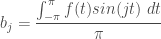
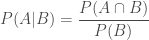
Its beauty is that it relates the probability of one event occurring after another to its inverse i.e. $P(A|B)$ or the probability of A after B, to $P(B|A)$ or the probability of B after A.

The standard example given in the textbooks is when $P(A)$ is the probability that an individual in a population has a disease, say cancer, and $P(B)$ is the probability that a medical test for that cancer comes back positive.

We are given, or can work out, the probability that any individual in the population has cancer (say 1%). We are also given the efficacy of the test i.e. the percentage of true positives the tests gives (I guess the manufacturer would provide this on the basis of trials, giving it to patients they know have cancer and patients they know don’t and then seeing how it performs. Say it’s 98%.) The manufacturers also give the number of false positives i.e. the number of times the test comes up positive and in fact there is no cancer (say 3%). So now imagine someone, imagine you in fact, take the cancer test and it comes up positive. What is the chance you have cancer?

Well, it’s not 99%.

But you can calculate the answer from the information given using Bayes’ Theorem. You want to know $P(A|B)$ , the probability of the test being positive after having cancer. Having gotten a positive test, having cancer is what you are frightened of. You have been given $P(B|A)$ which is the probability of having cancer after having the test (i.e. the efficacy of the test, the percentage of true positives, from the trials – 98% ). Bayes theorem allows you to relate the two.

The probabilities calculated are often surprising – much lower than most people would guess. In this instance it’s only 24.8%.

Unfortunately, if you just try and learn Bayes Theroem as some sort of magic formula into which you plug numbers, it’s very easy to get confused by all the $P(A)$ ‘s and $P(B)$ ‘s and $P(A|B)$ ‘s and so on, which is a shame because the basic ideas are quite straightforward.

Fortunately it’s also very easy to be come unconfused. When things are explained to you right.

In fact, as per usual, if you understand what is going with pictures, on you don’t need to learn any formulae at all. Just the pictures.

So here are the pictures.

Think of a sample space. We’re going to designate this by an empty rectangle. The rectangle represents every possible outcome for our experiments. Inside the rectangle we’re going to have 2 ovals, one for event A and one for event B. Oval A is blue. Oval B is yellow. Where oval A overlaps oval B is green. The size of each oval represents the probability of the event occuring i.e. if A is a huge oval almost filling the rectangle then this means A is very likely to happen. If we close our eyes and stick a pin inside the rectangle randomly, we are very likely to stick it inside the oval A. Similarly, if A is very small, the event A is unlikely to happen.

In order to understand Bayes Theroem there are only 3 scenarios we need consider.

Scenario 1

This is where if event B happens (i.e. you stick your pin in oval B) event A will never happen.

Imagine you hold an imaginary pin over the rectangle. You randomly plunge it down and, unfortunately, it sticks inside the oval B (unfortunately, because that is equivalent to getting your positive test result back). The moment the pin hits inside oval B, you shrink to the size of an ant and you find yourself standing inside oval B, exactly where your pin hit the paper. At the same time a ten foot high barbed wire fence suddenly shoots up around the boundary of oval B. The fence, not the rectangle, is now the limit of your world. You are frightened. You daren’t look down. Because if you look down and you see you are standing on a green carpet you know that means you have cancer. If you’re standing on a yellow carpet you’re safe – positive test, but no cancer.

What are the chances you are also standing on a green carpet? Well in this instance 0% – it can’t happen, because A is right over the other side of the rectangle and doesn’t connect with B at all. So you’re definitely safe.

This is the scenario with $P(A \cap B)$ = 0 i.e. where A and B don’t intersect. It gives $P(A|B)$ =0.

Now for scenario 2:

which is the scenario where B is right inside A.

So imagine again, you stuck your pin in the rectangle randomly and again you hit oval B (this time its totally green, because it’s all inside oval A). You tested positive. Again you shrink down to the size of an ant and find yourself standing where you stuck the pin. The ten foot high barbed wire fence shoots up around oval B, trapping you inside. You daren’t look down. What is the chance you’re standing on some green?

In this instance, you are definitely f*cked, because 100% of oval B is green.

$P(A \cap B) = P(B)$ gives $P(A|B)$ = 100%.

Finally scenario 3, the mixed case :

You plunge down your pin into the rectangle and, as always, are unlucky enough to stick it inside oval B. You shrink down to the size of an ant and stand up where the pin hit the oval. The fence shoots up around the boundary of oval B. You’re frightened to look down. What is the probability that you might be standing on green this time? Well, it’s not 100% nor 0% but something in between. Given a positive test it’s certainly possible you have cancer, but how possible?

In this case, some of the floor in the fenced off area is green, some is yellow. The probability you’re standing on green is the proportion of the green floor inside the fenced off area (all of the oval B).

$P(A|B) = \dfrac {P(A \cap B)} {P(B)}$ (i)

This is our general case. This formula also takes care of scenario 1 and scenario 2.

Now we want to go through the 3 scenarios again but this time imagining that when we plunged the pin down, we stuck it in oval A i.e. this time we definitely know we have cancer. We then take the test. What is the chance we are positive. So imagine jabbing the pin in oval A, and then shrinking to the size of an ant to stand where the pin hit the paper, and then the fence rising up around oval A, trapping you inside.

We could go through the whole rigmarole above, wondering what are the chances we are standing on blue or green.

Or we just swap the As and Bs around in the general formula (i) we already figured out.

This gives the other general case $P(B|A) = \dfrac {P(B \cap A)} {P(A)}$ (ii)

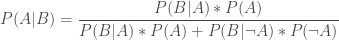
Now we know ${P(B \cap A)} = {P(A \cap B)}$ (check any of the scenario diagrams) so we can combine (i) and (ii), giving:

$P(A|B) = \dfrac {P(B|A) * P(A)} {P(B)}$

as per the neon lights.

This is the general form of the theorem, but we are not done yet because there is also a long form of the Theorem.

To get the long form, all we do is get rid of $P(B)$ from the bottom of the general formula. (In the original example, I didn’t give you $P(B)$ which would be the probability of a random person in the population testing positive either because they had cancer, or because of a false positive.)

To get rid of $P(B)$ we just look again at the mixed case (picture 3). Just think about the most bizarre way to describe $P(B)$ . In terms of intersections it is $P(A {\cap B})+P ({{\neg A} \cap B})$ where ${\neg A}$ stands for “not A”.

So using the formula (i) derived above $P(A|B) = \dfrac {P(A \cap B)} {P(B)}$ (i)

we can say $P(B|A) = \dfrac {P(B \cap A)} {P(A)}$ (which was our formula (ii), which we got by swapping A and B about)

and $P(B|{\neg A}) = \dfrac {P(B \cap \neg A)} {P(\neg A)}$ (swapping ${\neg A}$ for ${A}$ in formula (ii)).

So using our bizarre idea of $P(B)$ as $P(A {\cap B})+P ({{\neg A} \cap B})$ gives us a formula for $P(B) = {P(B|A) * P(A)} + {P(B| \neg A) * P( \neg A)}$

We use this in the original Bayes Formula as the denominator, giving the extended version:

$P(A|B) = \dfrac{P(B|A) * P(A)} {{P(B|A) * P(A)} + {P(B| \neg A) * P( \neg A)}}$

Questions using Bayes’ Theorem then become just exercises in plugging percentages to these formulae.

In our original example, $P(A)=0.01$ , $P(B|A)=0.98$ , $P(B| {\neg A}) = 0.03$ .

So using the extended formula $P(A|B) = \dfrac{({0.98} *{0.01})} {({0.98} * {0.01}) + {({0.03}* {0.99})}}$ = 24.8%.

There is hope – the chances of you having cancer after testing positive are not so dire after all.

Often using a table can be a good idea to make sure you have everything sorted out correctly. There are good examples of doing it like that here.

Movies I Quite Like

November 6, 2011February 4, 2012Leave a comment

I made a list. I’m checking it twice. I might add some more when I get around to it.

1. Enter the Void

Gasper Noé’s 2009 movie is the closest thing to a dream on celluloid we’re ever likely to see. Massively complex crane shots take us sweeping over a neon-lit Tokyo, as we follow the disembodied soul of small time drug dealer who has been shot and killed by the police. Long, difficult to watch at times, not afraid to be at turns sentimental and provocative, this is movie-making that attempts to push boundaries and move beyond straight-forward narrative to something more visceral.

2. King of Kong

The tale of a man who wishes to King of Kong – Donkey Kong that is, the old arcade game of rolling barrels and climbing ladders. Rather difficult you would have thought, and somewhat pointless, given the game has been out some thirty years now and no-one plays it any more. But you would be wrong. His quest exposes a whole sub-culture of bizarre individuals, not least of whom is Billy Mitchell, the “Video Game Player of the Century”, Dong Kong record holder, purveyor of “Rickey’s World Famous Sauces” and the only man ever to achieve a perfect score on Pacman. Would be totally unbelievable if it wasn’t true.

3. Dogville

A film that is shot on sound stage with chalk lines on the floor for walls, no scenery and minimal props shouldn’t work as a movie. But it undoubtedly does, thanks to some of the best acting you’re ever likely to see anywhere and a fantastic script by Lars van Trier that plays with conventions, gently lulling the audience into believing they know where a straightforward story is heading, and then carefully blowing their complacency apart.

4. Grizzly Man

Werner Herzog’s documentary uses Timothy Treadwell’s self-shot footage to tell the tale of a man who lived among, and was ultimately eaten by, grizzly bears. Treadwell emerges as a bizarre man-child who anthropomorphizes the bears, giving them name such as Mr Chocolate and Booble. He refuses to surround his tent with an electric fence, gets in trouble with the rangers for not taking basic precautions, camps where he wasn’t supposed to and talks in a weird affected Australian/English accent. Yet, you can’t help but like him. That he has a genuine bond and understanding with some of the bears is undeniable. His footage of them is incredible. And to be fair to him, his actual death seems to be a horrible accident – he was scheduled to leave the week before but stayed on and the bear that killed and ate him seems to have been a hungry rogue he was unfamiliar with. His girlfriend was eaten too.

5. Amelie

Everybody’s favourite French movie (except mine, if you count “Enter the Void” as French). Gentle comedy of this order nearly always fails to hit the mark, but Audrey Tatou gives a delightful performance in a role originally written for Emily Watson (thank God she was busy making Gosford Park.) The travelling gnome, the strange man in the photo booth, the sex in the toilets that nearly breaks all the café’s glasses – all the jokes have become strangely iconic. As has the movie.

6. City of God